\( \DeclareMathOperator{\abs}{abs} \newcommand{\ensuremath}[1]{\mbox{$#1$}} \)
Умова
| (%i88) | kill(all); |
\[\]\[\tag{%o0} \ensuremath{\mathrm{done}}\]
| (%i1) | load(draw)$ |
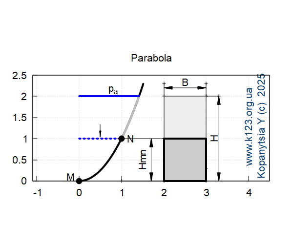
| (%i7) | ro:1000;g:9.81;H:2;B:3;Hmn:1;n:1000; |
\[\]\[\tag{%o2} 1000\]
\[\]\[\tag{%o3} 9.81\]
\[\]\[\tag{%o4} 2\]
\[\]\[\tag{%o5} 3\]
\[\]\[\tag{%o6} 1\]
\[\]\[\tag{%o7} 1000\]
| (%i12) | fh(x):=x··2;fHab(x):=Hmn;fH(x):=H;Fx(h):=sqrt(h);diff(Fx(h),h); |
\[\]\[\tag{%o8} \mathop{fh}(x)\mathop{:=}{{x}^{2}}\]
\[\]\[\tag{%o9} \mathop{fHab}(x)\mathop{:=}\ensuremath{\mathrm{Hmn}}\]
\[\]\[\tag{%o10} \mathop{fH}(x)\mathop{:=}H\]
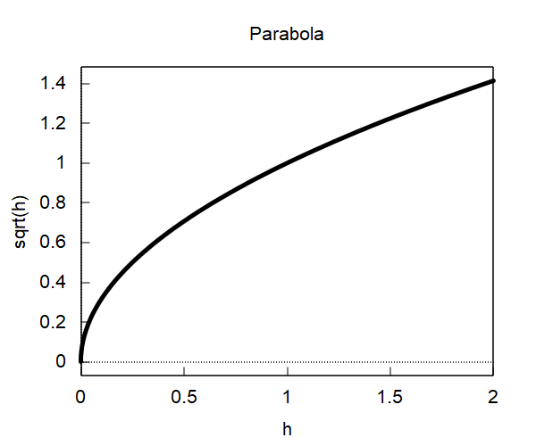
\[\]\[\tag{%o11} \mathop{Fx}(h)\mathop{:=}\sqrt{h}\]
\[\]\[\tag{%o12} \frac{1}{2 \sqrt{h}}\]
| (%i13) | dh(h):=1/(2·sqrt(h)); |
\[\]\[\tag{%o13} \mathop{dh}(h)\mathop{:=}\frac{1}{2 \sqrt{h}}\]
| (%i14) | Fx(1); |
\[\]\[\tag{%o14} 1\]
| (%i17) | del1:Hmn/10,numer;del2:Hmn/5,numer;del3:Hmn/3,numer; |
\[\]\[\tag{%o15} 0.1\]
\[\]\[\tag{%o16} 0.2\]
\[\]\[\tag{%o17} 0.3333333333333333\]
| (%i19) | del4:Hmn/2.5,numer;del5:Hmn/2,numer; |
\[\]\[\tag{%o18} 0.4\]
\[\]\[\tag{%o19} 0.5\]
| (%i20) | line_w:1; |
\[\]\[\tag{%o20} 1\]
| (%i21) |
draw2d(xrange = [−1.1,4.5], yrange = [0,2.5], font = "Arial", font_size = 16, title="Parabola", grid = true, proportional_axes=xy, line_width=4,color=black, explicit(fh(x),x,0,Fx(H)+del1), line_width=4,color=grey, explicit(fh(x),x,Hmn,Fx(H)), line_type = solid, line_width=3,color=blue, water:polygon([[0,H],[Fx(H),H]]), line_width=3,color=blue,line_type = dots, water_hm:polygon([[0,Hmn],[Fx(Hmn),Hmn]]), line_type = solid, color=black,line_width=1, head_both = true, head_length = 0.2, head_angle = 10, vector([H,H+del2],[1,0]), label(["B",2.5,H+del3]), points_joined = true, points([[2,2],[2,2.3]]), points([[3,2],[3,2.3]]), points([[3,2],[3.3,2]]), points([[3,0],[3,0.3]]), vector([3.3,0],[0,2]), points_joined = false, label_orientation = 'vertical, label(["H",3.2,Hmn]), points_joined = true, points([[Fx(Hmn),Hmn],[Fx(Hmn)+1,Hmn]]), points([[Fx(Hmn),0],[Fx(Hmn)+1,0]]), vector([Fx(Hmn)+0.7,0],[0,Hmn]), points_joined = false, label(["Hmn",1+0.5,Hmn/2]), color = black, label_orientation = 'horizontal, head_both = false, line_type = solid, head_length = 0.2, head_angle = 5, color = black, vector([0.5,(H+del3)],[0,−0.3]), label(["p_a",0.5+0.3,2+0.2]), color = black, fill_color = "#eeeeee", rectangle([2,0],[3,2]), color = black, fill_color = "#cccccc", line_width=4, rectangle([2,0],[3,1]), /* GPL */ font = "Arial", font_size = 16, color = "#0e406e", label_orientation = 'vertical, label(["www.k123.org.ua ",4,1.3]), label(["Kopanytsia Y (c) 2025",4.3,1.3]), color=black,point_type = filled_circle, point_size = 2, points_joined = false, points([[0,0]]), label_orientation = 'horizontal, label(["M",0−del2,0+del1]), points([[Hmn,Fx(Hmn)]]), label(["N",Hmn+del2,Fx(Hmn)]) )$ |

| (%i22) | plot2d([fh(x),fHab(x),fH(x)],[x,0,H]); |
\[\]\[\tag{%o22} false\]

| (%i23) | plot2d(Fx(h),[h,0,H], [color,black],[style, [lines, 5,5]]); |
\[\]\[\tag{%o23} false\]
| (%i24) | fp(h):=ro·g·(H−h); |
\[\]\[\tag{%o24} \mathop{fp}(h)\mathop{:=}\ensuremath{\mathrm{ro}} g\, \left( H\mathop{-}h\right) \]
| (%i25) | h_C_st:H−Hmn/2,numer; |
\[\]\[\tag{%o25} 1.5\]
| (%i26) | p_c_st:ro·g·h_C_st; |
\[\]\[\tag{%o26} 14715.0\]
| (%i27) | w_st:B·Hmn; |
\[\]\[\tag{%o27} 3\]
| (%i28) | P_x_st:p_c_st·w_st; |
\[\]\[\tag{%o28} 44145.0\]
| (%i29) | I:(B·Hmn··3)/12,numer; |
\[\]\[\tag{%o29} 0.25\]
| (%i30) | h_D_st:h_C_st+(I)/(h_C_st·w_st); |
\[\]\[\tag{%o30} 1.5555555555555556\]
| (%i31) | h_D_down_st:H−h_D_st; |
\[\]\[\tag{%o31} 0.4444444444444444\]
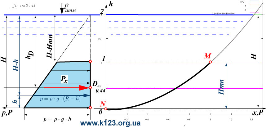
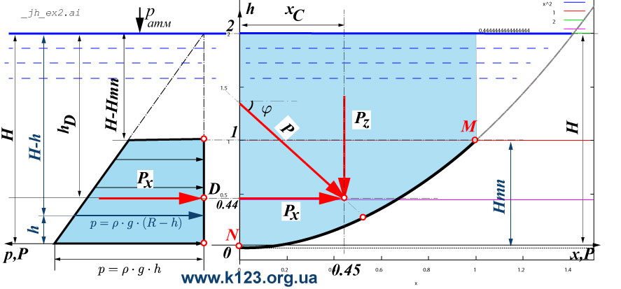
P_x - горизонтальна проекція сили тиску
| (%i32) | scale:100000; |
\[\]\[\tag{%o32} 100000\]
| (%i33) | P_x:integrate(fp(h)·B,h,0,Hmn); |
\[\]\[\tag{%o33} 44145.0\]
| (%i34) | mP_x:integrate(fp(h)·B·(H−h),h,0,Hmn); |
\[\]\[\tag{%o34} 68670.0\]
| (%i35) | mP_x_down:integrate(fp(h)·B·h,h,0,Hmn); |
\[\]\[\tag{%o35} 19620.0\]
| (%i36) | h_D:mP_x/P_x; |
\[\]\[\tag{%o36} 1.5555555555555556\]
| (%i37) | h_D_:mP_x_down/P_x; |
\[\]\[\tag{%o37} 0.4444444444444444\]
| (%i38) | h_D+h_D_; |
\[\]\[\tag{%o38} 2.0\]
| (%i39) | fv(y):=(2−0.25·y)/2; |
\[\]\[\tag{%o39} \mathop{fv}(y)\mathop{:=}\frac{2\mathop{-}0.25 y}{2}\]
| (%i42) | fv(0);fv(1);fv(2); |
\[\]\[\tag{%o40} 1\]
\[\]\[\tag{%o41} 0.875\]
\[\]\[\tag{%o42} 0.75\]
| (%i43) | integrate(ro_·g_·(H_−h)·B_,h,0,Hmn_); |
\[\]\[\tag{%o43} \mathop{-}\left( \frac{\ensuremath{\mathrm{B\_ }} \left( {{\ensuremath{\mathrm{Hmn\_ }}}^{2}}\mathop{-}2 \ensuremath{\mathrm{H\_ }} \ensuremath{\mathrm{Hmn\_ }}\right) \ensuremath{\mathrm{g\_ }} \ensuremath{\mathrm{ro\_ }}}{2}\right) \]
| (%i44) | P_plot(B_,x,H_):=−(4905.0·B_·(Hmn_^2−2·H_·Hmn_)); |
\[\]\[\tag{%o44} \mathop{P\_ plot}\left( \ensuremath{\mathrm{B\_ }}\mathop{,}x\mathop{,}\ensuremath{\mathrm{H\_ }}\right) \mathop{:=}\mathop{-}\left( 4905.0 \ensuremath{\mathrm{B\_ }} \left( {{\ensuremath{\mathrm{Hmn\_ }}}^{2}}\mathop{-}2 \ensuremath{\mathrm{H\_ }} \ensuremath{\mathrm{Hmn\_ }}\right) \right) \]
| (%i45) | P_plot(3,3,4); |
\[\]\[\tag{%o45} \mathop{-}\left( 14715.0 \left( {{\ensuremath{\mathrm{Hmn\_ }}}^{2}}\mathop{-}8 \ensuremath{\mathrm{Hmn\_ }}\right) \right) \]
| (%i46) | P_plot_(ro_,g_,B_,Hmn_,H_):=(−((B_·(Hmn_^2−2·H_·Hmn_)·g_·ro_)/2)); |
\[\]\[\tag{%o46} \mathop{P\_ plot\_ }\left( \ensuremath{\mathrm{ro\_ }}\mathop{,}\ensuremath{\mathrm{g\_ }}\mathop{,}\ensuremath{\mathrm{B\_ }}\mathop{,}\ensuremath{\mathrm{Hmn\_ }}\mathop{,}\ensuremath{\mathrm{H\_ }}\right) \mathop{:=}\mathop{-}\left( \frac{\ensuremath{\mathrm{B\_ }} \left( {{\ensuremath{\mathrm{Hmn\_ }}}^{2}}\mathop{-}2 \ensuremath{\mathrm{H\_ }} \ensuremath{\mathrm{Hmn\_ }}\right) \ensuremath{\mathrm{g\_ }} \ensuremath{\mathrm{ro\_ }}}{2}\right) \]
| (%i47) | P_plot_(1000,9.81,3,1,2); |
\[\]\[\tag{%o47} 44145.0\]
| (%i48) | integrate(ro·g·(H_−h)·B·h,h,0,Hmn_); |
\[\]\[\tag{%o48} \mathop{-}\left( 4905.0 \left( 2 {{\ensuremath{\mathrm{Hmn\_ }}}^{3}}\mathop{-}3 \ensuremath{\mathrm{H\_ }} {{\ensuremath{\mathrm{Hmn\_ }}}^{2}}\right) \right) \]
| (%i49) | mP_plot(x,H_):=−(4905.0·(2·x^3−3·H_·x^2)); |
\[\]\[\tag{%o49} \mathop{mP\_ plot}\left( x\mathop{,}\ensuremath{\mathrm{H\_ }}\right) \mathop{:=}\mathop{-}\left( 4905.0 \left( 2 {{x}^{3}}\mathop{-}3 \ensuremath{\mathrm{H\_ }} {{x}^{2}}\right) \right) \]
| (%i50) | integrate(ro_·g_·(H_−h_)·B_·h_,h_,0,Hmn_); |
\[\]\[\tag{%o50} \mathop{-}\left( \frac{\ensuremath{\mathrm{B\_ }} \left( 2 {{\ensuremath{\mathrm{Hmn\_ }}}^{3}}\mathop{-}3 \ensuremath{\mathrm{H\_ }} {{\ensuremath{\mathrm{Hmn\_ }}}^{2}}\right) \ensuremath{\mathrm{g\_ }} \ensuremath{\mathrm{ro\_ }}}{6}\right) \]
| (%i51) | tex(−((B_·(2·Hmn_^3−3·H_·Hmn_^2)·g_·ro_)/6),false); |
\[\]\[\tag{%o51} "\$ \$ -\backslash left(\{\{\{\backslash it B\backslash \_ \}\backslash ,\backslash left(2\backslash ,\{\backslash it Hmn\backslash \_ \}\textasciicircum3-3\backslash ,\{\backslash it H\backslash \_ \}\backslash , \{\backslash it Hmn\backslash \_ \}\textasciicircum2\backslash right)\backslash ,\{\backslash it g\backslash \_ \}\backslash ,\{\backslash it ro\backslash \_ \}\}\backslash over\{6\}\}\backslash right)\$ \$ "\]
| (%i52) | mP_plot_(ro_,g_,B_,Hmn_,H_):=(−(((2·Hmn_^3−3·H_·Hmn_^2)·g_·ro_)/2)); |
\[\]\[\tag{%o52} \mathop{mP\_ plot\_ }\left( \ensuremath{\mathrm{ro\_ }}\mathop{,}\ensuremath{\mathrm{g\_ }}\mathop{,}\ensuremath{\mathrm{B\_ }}\mathop{,}\ensuremath{\mathrm{Hmn\_ }}\mathop{,}\ensuremath{\mathrm{H\_ }}\right) \mathop{:=}\mathop{-}\left( \frac{\left( 2 {{\ensuremath{\mathrm{Hmn\_ }}}^{3}}\mathop{-}3 \ensuremath{\mathrm{H\_ }} {{\ensuremath{\mathrm{Hmn\_ }}}^{2}}\right) \ensuremath{\mathrm{g\_ }} \ensuremath{\mathrm{ro\_ }}}{2}\right) \]
| (%i53) | h_plot_D_(x,H_):=(−(4905.0·(2·x^3−3·H_·x^2)))/(−(14715.0·(x^2−2·H_·x))); |
\[\]\[\tag{%o53} \mathop{h\_ plot\_ D\_ }\left( x\mathop{,}\ensuremath{\mathrm{H\_ }}\right) \mathop{:=}\frac{\mathop{-}\left( 4905.0 \left( 2 {{x}^{3}}\mathop{-}3 \ensuremath{\mathrm{H\_ }} {{x}^{2}}\right) \right) }{\mathop{-}\left( 14715.0 \left( {{x}^{2}}\mathop{-}2 \ensuremath{\mathrm{H\_ }} x\right) \right) }\]
| (%i54) | rat((−(4905.0·(2·x^3−3·H_·x^2)))/(−(14715.0·(x^2−2·H_·x)))); |
\[\]\[rat: replaced 0.3333333333333333 by 1/3 = 0.3333333333333333\]
\[\]\[\tag{%o54)/R} \frac{2 {{x}^{2}}\mathop{-}3 \ensuremath{\mathrm{H\_ }} x}{3 x\mathop{-}6 \ensuremath{\mathrm{H\_ }}}\]
| (%i55) | h_plot_D(x,H_):=(2·x^2−3·H_·x)/(3·x−6·H_); |
\[\]\[\tag{%o55} \mathop{h\_ plot\_ D}\left( x\mathop{,}\ensuremath{\mathrm{H\_ }}\right) \mathop{:=}\frac{2 {{x}^{2}}\mathop{-}3 \ensuremath{\mathrm{H\_ }} x}{3 x\mathop{-}6 \ensuremath{\mathrm{H\_ }}}\]
| (%i56) | h_plot_D(3,4),numer; |
\[\]\[\tag{%o56} 1.2\]
| (%i57) | h_D_plot_(ro_,g_,B_,Hmn_,H_):=(−(((2·Hmn_^3−3·H_·Hmn_^2)·g_·ro_)/2))/((−((B_·(Hmn_^2−2·H_·Hmn_)·g_·ro_)/2))); |
\[\]\[\tag{%o57} \mathop{h\_ D\_ plot\_ }\left( \ensuremath{\mathrm{ro\_ }}\mathop{,}\ensuremath{\mathrm{g\_ }}\mathop{,}\ensuremath{\mathrm{B\_ }}\mathop{,}\ensuremath{\mathrm{Hmn\_ }}\mathop{,}\ensuremath{\mathrm{H\_ }}\right) \mathop{:=}\frac{\mathop{-}\left( \frac{\left( 2 {{\ensuremath{\mathrm{Hmn\_ }}}^{3}}\mathop{-}3 \ensuremath{\mathrm{H\_ }} {{\ensuremath{\mathrm{Hmn\_ }}}^{2}}\right) \ensuremath{\mathrm{g\_ }} \ensuremath{\mathrm{ro\_ }}}{2}\right) }{\mathop{-}\left( \frac{\ensuremath{\mathrm{B\_ }} \left( {{\ensuremath{\mathrm{Hmn\_ }}}^{2}}\mathop{-}2 \ensuremath{\mathrm{H\_ }} \ensuremath{\mathrm{Hmn\_ }}\right) \ensuremath{\mathrm{g\_ }} \ensuremath{\mathrm{ro\_ }}}{2}\right) }\]
| (%i58) | rat((−(((2·Hmn_^3−3·H_·Hmn_^2)·g_·ro_)/2))/(−((B_·(Hmn_^2−2·H_·Hmn_)·g_·ro_)/2))); |
\[\]\[\tag{%o58)/R} \frac{2 {{\ensuremath{\mathrm{Hmn\_ }}}^{2}}\mathop{-}3 \ensuremath{\mathrm{H\_ }} \ensuremath{\mathrm{Hmn\_ }}}{\ensuremath{\mathrm{B\_ }} \ensuremath{\mathrm{Hmn\_ }}\mathop{-}2 \ensuremath{\mathrm{B\_ }} \ensuremath{\mathrm{H\_ }}}\]
| (%i59) | _h_D_plot_(ro_,g_,B_,Hmn_,H_):=((2·Hmn_^2−3·H_·Hmn_)/(B_·Hmn_−2·B_·H_)); |
\[\]\[\tag{%o59} \mathop{\_ h\_ D\_ plot\_ }\left( \ensuremath{\mathrm{ro\_ }}\mathop{,}\ensuremath{\mathrm{g\_ }}\mathop{,}\ensuremath{\mathrm{B\_ }}\mathop{,}\ensuremath{\mathrm{Hmn\_ }}\mathop{,}\ensuremath{\mathrm{H\_ }}\right) \mathop{:=}\frac{2 {{\ensuremath{\mathrm{Hmn\_ }}}^{2}}\mathop{-}3 \ensuremath{\mathrm{H\_ }} \ensuremath{\mathrm{Hmn\_ }}}{\ensuremath{\mathrm{B\_ }} \ensuremath{\mathrm{Hmn\_ }}\mathop{-}2 \ensuremath{\mathrm{B\_ }} \ensuremath{\mathrm{H\_ }}}\]
| (%i60) | _h_D_plot_(1000,9.81,3,1,2),numer; |
\[\]\[\tag{%o60} 0.4444444444444444\]
| (%i61) | tex((2·Hmn_^2−3·H_·Hmn_)/(B_·Hmn_−2·B_·H_), false); |
\[\]\[\tag{%o61} "\$ \$ \{\{2\backslash ,\{\backslash it Hmn\backslash \_ \}\textasciicircum2-3\backslash ,\{\backslash it H\backslash \_ \}\backslash ,\{\backslash it Hmn\backslash \_ \}\}\backslash over\{\{\backslash it B\backslash \_ \}\backslash , \{\backslash it Hmn\backslash \_ \}-2\backslash ,\{\backslash it B\backslash \_ \}\backslash ,\{\backslash it H\backslash \_ \}\}\}\$ \$ "\]
| (%i65) | Ps:0;mPs:0;ni:10000;dhi:Hmn/ni; |
\[\]\[\tag{%o62} 0\]
\[\]\[\tag{%o63} 0\]
\[\]\[\tag{%o64} 10000\]
\[\]\[\tag{%o65} \frac{1}{10000}\]
| (%i66) | for i:1 thru ni step 1 do (Psi:ro·g·(H−dhi·i)·B·dhi,Ps:Ps+Psi)$ |
| (%i67) | for i:1 thru ni step 1 do (mPsi:ro·g·(H−dhi·i)·(dhi·i)·B·dhi,mPs:mPs+mPsi)$ |
| (%i70) | Ps;mPs;h_D_downi:mPs/Ps; |
\[\]\[\tag{%o68} 44143.528499999935\]
\[\]\[\tag{%o69} 19621.471450949975\]
\[\]\[\tag{%o70} 0.4444925930864363\]
| (%i71) | P_xv:P_x/scale; |
\[\]\[\tag{%o71} 0.44145\]
| (%i72) |
draw2d(xrange = [−1.1,4.5], yrange = [0,3], font = "Arial", font_size = 16, title="Parabola", grid = true, proportional_axes=xy, line_width=4,color=black, explicit(fh(x),x,0,Fx(H)+del1), line_width=4,color=grey, explicit(fh(x),x,Hmn,Fx(H)), line_type = solid, line_width=3,color=blue, water:polygon([[0,H],[Fx(H),H]]), line_width=3,color=blue,line_type = dots, water_hm:polygon([[0,Hmn],[Fx(Hmn),Hmn]]), line_type = solid, color=black,line_width=1, head_both = true, head_length = 0.2, head_angle = 10, vector([H,H+del2],[1,0]), label(["B",2.5,H+del3]), points_joined = true, points([[2,2],[2,2.3]]), points([[3,2],[3,2.3]]), points([[3,2],[3.3,2]]), points([[3,0],[3,0.3]]), vector([3.3,0],[0,2]), points_joined = false, label_orientation = 'vertical, label(["H",3.2,Hmn]), points_joined = true, points([[Fx(Hmn),Hmn],[Fx(Hmn)+1,Hmn]]), points([[Fx(Hmn),0],[Fx(Hmn)+1,0]]), vector([Fx(Hmn)+0.7,0],[0,Hmn]), points_joined = false, label(["Hmn",1+0.5,Hmn/2]), color = black, label_orientation = 'horizontal, head_both = false, line_type = solid, head_length = 0.2, head_angle = 5, color = black, vector([0.5,(H+del3)],[0,−del3]), label(["p_a",0.5+del3,H+del2]), color = black, fill_color = "#eeeeee", rectangle([2,0],[3,2]), color = black, fill_color = "#cccccc", line_width=4, rectangle([2,0],[3,1]), /* GPL */ font = "Arial", font_size = 16, color = "#0e406e", label_orientation = 'vertical, label(["www.k123.org.ua ",4,1.3]), label(["Kopanytsia Y (c) 2025",4.3,1.3]), color=black,point_type = filled_circle, point_size = 2, points_joined = false, points([[0,0]]), label_orientation = 'horizontal, label(["M",0−del2,0+del1]), points([[Hmn,Fx(Hmn)]]), label(["N",Hmn+del2,Fx(Hmn)]), /* Epura */ line_width=1,color=blue,line_type = short_long_dashes, fill_color = "#ffffff", poly:polygon([[0−0.1,0],[0−0.1,2],[−1−0.1,0],[0−0.1,0]]), line_width=1,color=blue,line_type = solid, fill_color = lightblue, poly:polygon([[0−0.1,0],[0−0.1,1],[−0.5−0.1,1],[−1−0.1,0],[0−0.1,0]]), line_type = solid, head_length = 0.3, head_angle = 5, color = blue, line_width=3, vector([−fv(0)−0.05,0],[fv(0)−0.05,0]), vector([−fv(1)−0.05,0.25],[fv(1)−0.05,0]), vector([−fv(2)−0.05,0.5],[fv(2)−0.05,0]), vector([−fv(3)−0.05,0.75],[fv(3)−0.05,0]), vector([−fv(4)−0.05,1],[fv(4)−0.05,0]), color = red, label(["Px",0,h_D_+del2]), label(["0.44",0−0.8,h_D_]), line_type = solid, head_length = 0.2, head_angle = 5, line_width=2, vector([0−P_xv−del1,h_D_],[P_xv,0]), points([[0−del1,h_D_]]), points_joined = true, line_width=0.5, point_size = 0.1, points([[−1,h_D_],[4,h_D_]]), points([[2.5,0],[2.5,H]]), label_orientation = 'vertical, head_both = true, line_type = solid, head_length = 0.2, head_angle = 5, vector([1,h_D_],[0,−h_D_]), label(["h_D",1−del2,h_D_/2]), /* label_orientation = 'horizontal, label(["h_D = 0.56 m, P_x=44145.0 N",2,Hmn+del3]), */ fill_color = white, rectangle([0,3−del4],[4,3]), label_orientation = 'vertical, head_both = true, line_type = solid, head_length = 0.2, head_angle = 5, label_orientation = 'horizontal, label(["h_D = 0.44 m, P_x=44145.0",2,3−del2]) )$ |
| --> | h_D;P_x; |
\[\]\[\tag{%o35} 0.6111111111111112\]
\[\]\[\tag{%o36} 44145.0\]

P_x - чисельний алгоритм методу К123
| (%i75) | P_x_sum:0;dh:Hmn/n;h:0; |
\[\]\[\tag{%o73} 0\]
\[\]\[\tag{%o74} \frac{1}{1000}\]
\[\]\[\tag{%o75} 0\]
| (%i76) | Pi_x(h):=ro·g·(H−h)·B; |
\[\]\[\tag{%o76} \mathop{Pi\_ x}(h)\mathop{:=}\ensuremath{\mathrm{ro}} g\, \left( H\mathop{-}h\right) B\]
| (%i78) | for i:1 while h < Hmn do (Pi:Pi_x(h)·dh,P_x_sum:P_x_sum+Pi,h:h+dh);P_x_:P_x_sum; |
\[\]\[\tag{%o77} \ensuremath{\mathrm{done}}\]
\[\]\[\tag{%o78} 44159.71499999999\]
| (%i79) | Px_test:integrate(Pi_x(hi),hi,0,Hmn); |
\[\]\[\tag{%o79} 44145.0\]
| (%i82) | mP_x_sum:0;dh:Hmn/n;h:0; |
\[\]\[\tag{%o80} 0\]
\[\]\[\tag{%o81} \frac{1}{1000}\]
\[\]\[\tag{%o82} 0\]
| (%i84) | for i:1 while h < Hmn do (Pi:Pi_x(h)·dh·h,mP_x_sum:mP_x_sum+Pi,h:h+dh);mP_x_:mP_x_sum; |
\[\]\[\tag{%o83} \ensuremath{\mathrm{done}}\]
\[\]\[\tag{%o84} 19605.280095000024\]
| (%i85) | kill(h); |
\[\]\[\tag{%o85} \ensuremath{\mathrm{done}}\]
| (%i86) | mPx_test:integrate(Pi_x(h)·(h),h,0,Hmn); |
\[\]\[\tag{%o86} 19620.0\]
| (%i88) | h_D:mP_x_sum/P_x_sum;h_D_test:mPx_test/Px_test; |
\[\]\[\tag{%o87} 0.44396301232922425\]
\[\]\[\tag{%o88} 0.4444444444444444\]
| (%i89) | Rel_ERROR:(100/h_D_test)·(h_D_test−h_D),numer; |
\[\]\[\tag{%o89} 0.10832222592453838\]
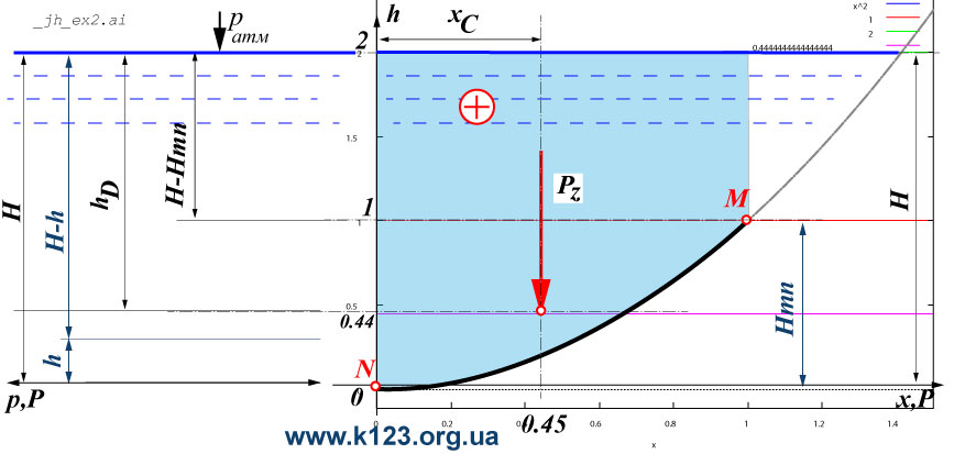
P_z - вертикальна проекція сили тиску
| (%i90) | kill(h); |
\[\]\[\tag{%o90} \ensuremath{\mathrm{done}}\]
| (%i95) | ro:1000;g:9.81;H:2;B:3;Hmn:1; |
\[\]\[\tag{%o91} 1000\]
\[\]\[\tag{%o92} 9.81\]
\[\]\[\tag{%o93} 2\]
\[\]\[\tag{%o94} 3\]
\[\]\[\tag{%o95} 1\]
| (%i96) | P_z:integrate(fp(h)·B·dh(h),h,0,Hmn); |
\[\]\[\tag{%o96} 49050.0\]
| (%i97) | mP_z:integrate(fp(h)·B·dh(h)·(Fx(h)),h,0,Hmn); |
\[\]\[\tag{%o97} 22072.5\]
| (%i98) | x_C:mP_z/P_z; |
\[\]\[\tag{%o98} 0.45\]
| (%i99) | integrate(ro_·g_·(H_−h_)·B_·(1/(2·sqrt(h_))),h_,0,Hmn_); |
\[\]\[\mbox{}\\"Is "\ensuremath{\mathrm{Hmn\_ }}" positive, negative or zero?"positive;\]
\[\]\[\tag{%o99} \mathop{-}\left( \frac{\ensuremath{\mathrm{B\_ }} \sqrt{\ensuremath{\mathrm{Hmn\_ }}} \left( 2 \ensuremath{\mathrm{Hmn\_ }}\mathop{-}6 \ensuremath{\mathrm{H\_ }}\right) \ensuremath{\mathrm{g\_ }} \ensuremath{\mathrm{ro\_ }}}{6}\right) \]
| (%i100) | Pz(ro_,g_,B_,Hmn_,H_):=−((B_·sqrt(Hmn_)·(2·Hmn_−6·H_)·g_·ro_)/6); |
\[\]\[\tag{%o100} \mathop{Pz}\left( \ensuremath{\mathrm{ro\_ }}\mathop{,}\ensuremath{\mathrm{g\_ }}\mathop{,}\ensuremath{\mathrm{B\_ }}\mathop{,}\ensuremath{\mathrm{Hmn\_ }}\mathop{,}\ensuremath{\mathrm{H\_ }}\right) \mathop{:=}\mathop{-}\left( \frac{\ensuremath{\mathrm{B\_ }} \sqrt{\ensuremath{\mathrm{Hmn\_ }}} \left( 2 \ensuremath{\mathrm{Hmn\_ }}\mathop{-}6 \ensuremath{\mathrm{H\_ }}\right) \ensuremath{\mathrm{g\_ }} \ensuremath{\mathrm{ro\_ }}}{6}\right) \]
| (%i101) | Pz(1000,9.81,3,1,2); |
\[\]\[\tag{%o101} 49050.0\]
| (%i110) | integrate(ro_·g_·(H_−h_)·B_·(1/(2·sqrt(h_)))·sqrt(h_),h_,0,Hmn_); |
\[\]\[\tag{%o110} \mathop{-}\left( \frac{\ensuremath{\mathrm{B\_ }} \left( {{\ensuremath{\mathrm{Hmn\_ }}}^{2}}\mathop{-}2 \ensuremath{\mathrm{H\_ }} \ensuremath{\mathrm{Hmn\_ }}\right) \ensuremath{\mathrm{g\_ }} \ensuremath{\mathrm{ro\_ }}}{4}\right) \]
| (%i111) | mPz(ro_,g_,B_,Hmn_,H_):=−((B_·(Hmn_^2−2·H_·Hmn_)·g_·ro_)/4); |
\[\]\[\tag{%o111} \mathop{mPz}\left( \ensuremath{\mathrm{ro\_ }}\mathop{,}\ensuremath{\mathrm{g\_ }}\mathop{,}\ensuremath{\mathrm{B\_ }}\mathop{,}\ensuremath{\mathrm{Hmn\_ }}\mathop{,}\ensuremath{\mathrm{H\_ }}\right) \mathop{:=}\mathop{-}\left( \frac{\ensuremath{\mathrm{B\_ }} \left( {{\ensuremath{\mathrm{Hmn\_ }}}^{2}}\mathop{-}2 \ensuremath{\mathrm{H\_ }} \ensuremath{\mathrm{Hmn\_ }}\right) \ensuremath{\mathrm{g\_ }} \ensuremath{\mathrm{ro\_ }}}{4}\right) \]
| (%i112) | fx_C(ro_,g_,B_,Hmn_,H_):=(−((B_·(Hmn_^2−2·H_·Hmn_)·g_·ro_)/4))/(−((B_·sqrt(Hmn_)·(2·Hmn_−6·H_)·g_·ro_)/6)); |
\[\]\[\tag{%o112} \mathop{fx\_ C}\left( \ensuremath{\mathrm{ro\_ }}\mathop{,}\ensuremath{\mathrm{g\_ }}\mathop{,}\ensuremath{\mathrm{B\_ }}\mathop{,}\ensuremath{\mathrm{Hmn\_ }}\mathop{,}\ensuremath{\mathrm{H\_ }}\right) \mathop{:=}\frac{\mathop{-}\left( \frac{\ensuremath{\mathrm{B\_ }} \left( {{\ensuremath{\mathrm{Hmn\_ }}}^{2}}\mathop{-}2 \ensuremath{\mathrm{H\_ }} \ensuremath{\mathrm{Hmn\_ }}\right) \ensuremath{\mathrm{g\_ }} \ensuremath{\mathrm{ro\_ }}}{4}\right) }{\mathop{-}\left( \frac{\ensuremath{\mathrm{B\_ }} \sqrt{\ensuremath{\mathrm{Hmn\_ }}} \left( 2 \ensuremath{\mathrm{Hmn\_ }}\mathop{-}6 \ensuremath{\mathrm{H\_ }}\right) \ensuremath{\mathrm{g\_ }} \ensuremath{\mathrm{ro\_ }}}{6}\right) }\]
| (%i113) | rat((−((B_·(Hmn_^2−2·H_·Hmn_)·g_·ro_)/4))/(−((B_·sqrt(Hmn_)·(2·Hmn_−6·H_)·g_·ro_)/6))); |
\[\]\[\tag{%o113)/R} \frac{3 {{\ensuremath{\mathrm{Hmn\_ }}}^{2}}\mathop{-}6 \ensuremath{\mathrm{H\_ }} \ensuremath{\mathrm{Hmn\_ }}}{4 \sqrt{\ensuremath{\mathrm{Hmn\_ }}} \ensuremath{\mathrm{Hmn\_ }}\mathop{-}12 \ensuremath{\mathrm{H\_ }} \sqrt{\ensuremath{\mathrm{Hmn\_ }}}}\]
| (%i114) | x_C(ro_,g_,B_,Hmn_,H_):=((3·Hmn_^2−6·H_·Hmn_)/(4·sqrt(Hmn_)·Hmn_−12·H_·sqrt(Hmn_))); |
\[\]\[\tag{%o114} \mathop{x\_ C}\left( \ensuremath{\mathrm{ro\_ }}\mathop{,}\ensuremath{\mathrm{g\_ }}\mathop{,}\ensuremath{\mathrm{B\_ }}\mathop{,}\ensuremath{\mathrm{Hmn\_ }}\mathop{,}\ensuremath{\mathrm{H\_ }}\right) \mathop{:=}\frac{3 {{\ensuremath{\mathrm{Hmn\_ }}}^{2}}\mathop{-}6 \ensuremath{\mathrm{H\_ }} \ensuremath{\mathrm{Hmn\_ }}}{4 \sqrt{\ensuremath{\mathrm{Hmn\_ }}} \ensuremath{\mathrm{Hmn\_ }}\mathop{-}12 \ensuremath{\mathrm{H\_ }} \sqrt{\ensuremath{\mathrm{Hmn\_ }}}}\]
| (%i116) | x_C(1000,9.81,3,1,2),numer; |
\[\]\[\tag{%o116} 0.45\]
| (%i103) | dh(h);Fx(h); |
\[\]\[\tag{%o102} \frac{1}{2 \sqrt{h}}\]
\[\]\[\tag{%o103} \sqrt{h}\]
| --> | P_zv:P_z/scale; |
\[\]\[\tag{%o70} 0.4905\]
| --> | ytop=3; |
\[\]\[\tag{%o71} \ensuremath{\mathrm{ytop}}\mathop{=}3\]
| --> |
draw2d(xrange = [−1.1,4.5], yrange = [0,3], font = "Arial", font_size = 16, title="Parabola", grid = true, proportional_axes=xy, /* vertical W */ line_width=0.5, color=blue, fill_color = lightblue, Wall:polygon([[0,0],[0,2],[1,2],[1,1],[0.75,0.75··2],[0.5,0.5··2],[0.25,0.25··2],[0,0]]), W:polygon([[0,0],[0,2]]), W:polygon([[0.25,0.25··2],[0.25,2]]), W:polygon([[0.5,0.5··2],[0.5,2]]), W:polygon([[0.75,0.75··2],[0.75,2]]), W:polygon([[1,1··2],[1,2]]), /* -- the end W */ line_width=4,color=black, explicit(fh(x),x,0,Fx(H)+del1), line_width=4,color=grey, explicit(fh(x),x,Hmn,Fx(H)), line_type = solid, line_width=3,color=blue, water:polygon([[0,H],[Fx(H),H]]), line_width=3,color=blue,line_type = dots, water_hm:polygon([[0,Hmn],[Fx(Hmn),Hmn]]), line_type = solid, color=black,line_width=1, head_both = true, head_length = 0.2, head_angle = 10, vector([H,H+del2],[1,0]), label(["B",2.5,H+del3]), points_joined = true, points([[2,2],[2,2.3]]), points([[3,2],[3,2.3]]), points([[3,2],[3.3,2]]), points([[3,0],[3,0.3]]), vector([3.3,0],[0,2]), points_joined = false, label_orientation = 'vertical, label(["H",3.2,Hmn]), points_joined = true, points([[Fx(Hmn),Hmn],[Fx(Hmn)+1,Hmn]]), points([[Fx(Hmn),0],[Fx(Hmn)+1,0]]), vector([Fx(Hmn)+0.7,0],[0,Hmn]), points_joined = false, label(["Hmn",1+0.5,Hmn/2]), color = black, label_orientation = 'horizontal, head_both = false, line_type = solid, head_length = 0.2, head_angle = 5, color = black, vector([0.8,(H+del3)],[0,−del3]), label(["p_a",0.8+del3,H+del2]), color = black, fill_color = "#eeeeee", rectangle([2,0],[3,2]), color = black, fill_color = "#cccccc", line_width=4, rectangle([2,0],[3,1]), /* GPL */ font = "Arial", font_size = 16, color = "#0e406e", label_orientation = 'vertical, label(["www.k123.org.ua ",4,1.3]), label(["Kopanytsia Y (c) 2025",4.3,1.3]), color=black,point_type = filled_circle, point_size = 2, points_joined = false, points([[0,0]]), label_orientation = 'horizontal, label(["M",0−del2,0+del1]), points([[Hmn,Fx(Hmn)]]), label(["N",Hmn+del2,Fx(Hmn)]), /* Epura line_width=1,color=blue,line_type = short_long_dashes, fill_color = "#ffffff", poly:polygon([[0−0.1,0],[0−0.1,2],[−1−0.1,0],[0−0.1,0]]), line_width=1,color=blue,line_type = solid, fill_color = lightblue, poly:polygon([[0−0.1,0],[0−0.1,1],[−0.5−0.1,1],[−1−0.1,0],[0−0.1,0]]), line_type = solid, head_length = 0.3, head_angle = 5, color = blue, line_width=3, vector([−fv(0)−0.05,0],[fv(0)−0.05,0]), vector([−fv(1)−0.05,0.25],[fv(1)−0.05,0]), vector([−fv(2)−0.05,0.5],[fv(2)−0.05,0]), vector([−fv(3)−0.05,0.75],[fv(3)−0.05,0]), vector([−fv(4)−0.05,1],[fv(4)−0.05,0]), color = red, label(["Px",0,h_D+del2]), label(["0.56",0-0.8,h_D]), line_type = solid, head_length = 0.2, head_angle = 5, line_width=2, vector([0−P_xv-del1,h_D],[P_xv,0]), points([[0-del1,h_D]]), points_joined = true, line_width=0.5, point_size = 0.1, points([[-1,h_D],[4,h_D]]), points([[2.5,0],[2.5,H]]), label_orientation = 'vertical, head_both = true, line_type = solid, head_length = 0.2, head_angle = 5, vector([1,h_D],[0,-h_D]), label(["h_D",1-del2,h_D/2]), */ /* label_orientation = 'vertical, color = "#654321", label(["Vertical orientation",x_C-0.2,h_D+0.6]), */ label_orientation = 'vertical, color = red, label(["Pz",x_C−0.1,h_D+0.4]), line_type = solid, head_length = 0.2, head_angle = 5, line_width=1.5, vector([x_C,(h_D+P_zv)],[0,−(P_zv)]), label_orientation = 'horizontal, color = red, line_type = solid, line_width=1, head_both = true, head_length = 0.2, head_angle = 10, vector([0,H+del2],[x_C,0]), label(["x_C",x_C/2,H+del3+del1]), points_joined = true, point_size = 0.1, line_type = solid, points([[0,H],[0,H+del3]]), line_type = dashes, points([[x_C,0],[x_C,H+del3]]), fill_color = white, rectangle([0,3−del4],[4,3]), label_orientation = 'vertical, head_both = true, line_type = solid, head_length = 0.2, head_angle = 5, label_orientation = 'horizontal, label(["x_C = 0.45 m, P_z=49050.0 N",2,3−del2]), label(["0.45",x_C,del1]) )$ |
| --> | x_C;P_z; |
\[\]\[\tag{%o69} 0.45\]
\[\]\[\tag{%o70} 49050.0\]

P_z - чисельний алгоритм методу К123
| --> | ro:1000;g:9.81;H:2;B:3;Hmn:1; |
\[\]\[\tag{%o73} 1000\]
\[\]\[\tag{%o74} 9.81\]
\[\]\[\tag{%o75} 2\]
\[\]\[\tag{%o76} 3\]
\[\]\[\tag{%o77} 1\]
| --> | P_z_sum:0;dh:Hmn/n;h:0; |
\[\]\[\tag{%o78} 0\]
\[\]\[\tag{%o79} \frac{1}{1000}\]
\[\]\[\tag{%o80} 0\]
| --> | fB(i,dh):=sqrt(i·dh); fB(1,dh),numer; |
\[\]\[\tag{%o81} \mathop{fB}\left( i\mathop{,}\ensuremath{\mathrm{dh}}\right) \mathop{:=}\sqrt{i\, \ensuremath{\mathrm{dh}}}\]
\[\]\[\tag{%o82} 0.03162277660168379\]
| --> | Pi_x(h):=ro·g·(H−h)·B; Pi_x(0.2); |
\[\]\[\tag{%o83} \mathop{Pi\_ x}(h)\mathop{:=}\ensuremath{\mathrm{ro}} g\, \left( H\mathop{-}h\right) B\]
\[\]\[\tag{%o84} 52974.0\]
| --> | fdb(i,dh):=(fB((i+1),dh)−fB((i),dh))/dh;fdb(1000,dh),numer; |
\[\]\[\tag{%o85} \mathop{fdb}\left( i\mathop{,}\ensuremath{\mathrm{dh}}\right) \mathop{:=}\frac{\mathop{fB}\left( i\mathop{+}1\mathop{,}\ensuremath{\mathrm{dh}}\right) \mathop{-}\mathop{fB}\left( i\mathop{,}\ensuremath{\mathrm{dh}}\right) }{\ensuremath{\mathrm{dh}}}\]
\[\]\[\tag{%o86} 0.4998750624609638\]
| --> | for i: 0 while h < Hmn do (db:fdb(i,dh),Pi:Pi_x(h)·db·dh,P_z_sum:P_z_sum+Pi,h:h+dh)$ |
| --> | P_z_:P_z_sum,numer;h; |
\[\]\[\tag{%o88} 49064.52275520602\]
\[\]\[\tag{%o89} 1\]
| --> | mP_z_sum:0;dh:Hmn/n;h:0; |
\[\]\[\tag{%o90} 0\]
\[\]\[\tag{%o91} \frac{1}{1000}\]
\[\]\[\tag{%o92} 0\]
| --> | for i: 0 while h < Hmn do (db:fdb(i,dh),Pi:Pi_x(h)·db·dh·fB(i,dh),mP_z_sum:mP_z_sum+Pi,h:h+dh)$ |
| --> | mP_z_:mP_z_sum,numer;h; |
\[\]\[\tag{%o94} 22003.335303355238\]
\[\]\[\tag{%o95} 1\]
| --> | x_C_:mP_z_/P_z_,numer; x_C; |
\[\]\[\tag{%o96} 0.44845713496765977\]
\[\]\[\tag{%o97} 0.45\]
| --> | Rel_ERROR:(100/x_C)·(x_C−x_C_),numer; |
\[\]\[\tag{%o98} 0.3428588960756102\]
P - Сила гідростатичного тиску
| --> | P_x;P_z; |
\[\]\[\tag{%o99} 44145.0\]
\[\]\[\tag{%o100} 49050.0\]
| --> | P:sqrt(P_x··2+P_z··2); |
\[\]\[\tag{%o101} 65990.02595089655\]
| --> | phi_rad:atan(P_z/P_x),numer; |
\[\]\[\tag{%o102} 0.83798122500839\]
| --> | phi_grad:atan(P_z/P_x)·(180/%pi),numer; |
\[\]\[\tag{%o103} 48.01278750418334\]
| --> | d:tan(P_z/P_x); |
\[\]\[\tag{%o104} 2.0199703317182265\]
| --> | k:P_z/P_x; |
\[\]\[\tag{%o105} 1.1111111111111112\]
| --> | scale:100000; |
\[\]\[\tag{%o106} 100000\]
| --> | P_xv:P_x/scale;P_zv:P_z/scale;Pv:P/scale; |
\[\]\[\tag{%o107} 0.44145\]
\[\]\[\tag{%o108} 0.4905\]
\[\]\[\tag{%o109} 0.6599002595089656\]
| --> | kill(D); |
\[\]\[\tag{%o110} \ensuremath{\mathrm{done}}\]
| --> | h_D;x_C;phi_rad;k; |
\[\]\[\tag{%o111} 0.44396301232922425\]
\[\]\[\tag{%o112} 0.45\]
\[\]\[\tag{%o113} 0.83798122500839\]
\[\]\[\tag{%o114} 1.1111111111111112\]
| --> | eq:h_D=−k·x_C+D; |
\[\]\[\tag{%o106} 0.44396301232922425\mathop{=}D\mathop{-}0.5\]
| --> | Di:h_D+k·x_C; |
\[\]\[\tag{%o115} 0.9439630123292242\]
| --> | solve(eq,D); |
\[\]\[rat: replaced 0.9439630123292242 by 2832833/3001000 = 0.9439630123292236\]
\[\]\[\tag{%o107} \left[ D\mathop{=}\frac{2832833}{3001000}\right] \]
| --> | D:2832833/3001000,numer; |
\[\]\[\tag{%o108} 0.9439630123292236\]
| --> | y(x):=−k·x+D; |
\[\]\[\tag{%o109} \mathop{y}(x)\mathop{:=}\mathop{-}k x\mathop{+}D\]
| --> | y(0.45); |
\[\]\[\tag{%o110} 0.44396301232922364\]
| --> | y1(x):=x··2; |
\[\]\[\tag{%o111} \mathop{y1}(x)\mathop{:=}{{x}^{2}}\]
| --> | eq1:−k·x+D=x··2; |
\[\]\[\tag{%o112} 0.9439630123292236\mathop{-}1.1111111111111112 x\mathop{=}{{x}^{2}}\]
| --> | solutions:solve([eq1],[x]); |
\[\]\[rat: replaced 0.9439630123292236 by 2832833/3001000 = 0.9439630123292236 \]\[rat: replaced -1.1111111111111112 by -10/9 = -1.1111111111111112\]
\[\]\[\tag{%o113} \left[ x\mathop{=}\mathop{-}\left( \frac{\sqrt{9137579034730}\mathop{+}1500500}{2700900}\right) \mathop{,}x\mathop{=}\frac{\sqrt{9137579034730}\mathop{-}1500500}{2700900}\right] \]
| --> | xvals: map(rhs, solutions); |
\[\]\[\tag{%o114} \left[ \mathop{-}\left( \frac{\sqrt{9137579034730}\mathop{+}1500500}{2700900}\right) \mathop{,}\frac{\sqrt{9137579034730}\mathop{-}1500500}{2700900}\right] \]
| --> | x_coord:xvals[2],numer; |
\[\]\[\tag{%o115} 0.5636428127589562\]
| --> | h_coord:y1(x_coord); |
\[\]\[\tag{%o116} 0.3176932203748278\]
| --> | xx:x_coord−P_xv;hh:h_coord+P_zv; |
\[\]\[\tag{%o117} 0.12219281275895622\]
\[\]\[\tag{%o118} 0.8081932203748278\]
| --> | f1(x):=−k·x+Di;f2(x):=x··2;h1:0;h2:0;ni:1000;x1:0;x2:sqrt(Hmn);xi:x2/ni;j:0; |
\[\]\[\tag{%o218} \mathop{f1}(x)\mathop{:=}\mathop{-}k x\mathop{+}\ensuremath{\mathrm{Di}}\]
\[\]\[\tag{%o219} \mathop{f2}(x)\mathop{:=}{{x}^{2}}\]
\[\]\[\tag{%o220} 0\]
\[\]\[\tag{%o221} 0\]
\[\]\[\tag{%o222} 1000\]
\[\]\[\tag{%o223} 0\]
\[\]\[\tag{%o224} 1\]
\[\]\[\tag{%o225} \frac{1}{1000}\]
\[\]\[\tag{%o226} 0\]
| --> | Di;f1(xi·1000),numer;f2(xi·1000),numer; |
\[\]\[\tag{%o233} 0.9439630123292242\]
\[\]\[\tag{%o234} \mathop{-}0.16714809878188697\]
\[\]\[\tag{%o235} 1.0\]
| --> | for j: 1 while f1(xi·j)−f2(xi·j)>0 do (j: j+1,x2:xi·j); |
\[\]\[\tag{%o241} \ensuremath{\mathrm{done}}\]
| --> | x2,numer; |
\[\]\[\tag{%o244} 0.564\]
| --> |
plot2d([y1(x),y(x),[discrete,[x_coord],[h_coord]], [discrete,[x_coord,xx],[h_coord,hh]], [discrete,[x_coord,xx],[h_coord,h_coord]], [discrete,[x_coord,x_coord],[h_coord,hh]], [discrete,[0,2],[2,2]]],[x,0,2.1],[y,0,2.1], [style, [lines, 5,5], [lines, 3,1], [points, 5,2],[lines, 3,2],[lines, 3,2],[lines, 3,2], [lines, 3,1]]); |
\[\]\[\] \texttt{%error plot2d: expression evaluates to non-numeric value everywhere in plotting range. }\[\]\[\] \texttt{%error plot2d: expression evaluates to non-numeric value everywhere in plotting range. }\[\]\[\] \texttt{%error Warning: none of the points have numerical values. }\[\]\[\] \texttt{%error Warning: none of the points have numerical values. }\[\]\[\] \texttt{%error Warning: none of the points have numerical values. }\[\]\[\] \texttt{%error Warning: none of the points have numerical values.}\[\]
\[\]\[\tag{%o245} false\]

Draw
| --> | /* y = 1-1-4 */; |
| --> | fv(y):=(2−0.25·y)/2; |
\[\]\[\tag{%o120} \mathop{fv}(y)\mathop{:=}\frac{2\mathop{-}0.25 y}{2}\]
| --> |
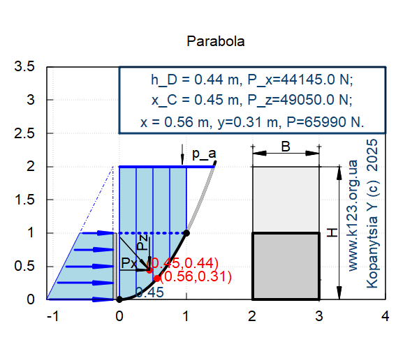
draw2d(xrange = [−1.1,4], yrange = [0,3.5], font = "Arial", font_size = 16, title="Parabola", grid = true, proportional_axes=xy, /* vertical W */ fill_color = lightblue, Wall:polygon([[0,0],[0,2],[1,2],[1,1],[0.75,0.75··2],[0.5,0.5··2],[0.25,0.25··2],[0,0]]), W:polygon([[0,0],[0,2]]), W:polygon([[0.25,0.25··2],[0.25,2]]), W:polygon([[0.5,0.5··2],[0.5,2]]), W:polygon([[0.75,0.75··2],[0.75,2]]), W:polygon([[1,1··2],[1,2]]), line_width=4,color=black, explicit(y1(x),x,0,1.44), line_width=4,color=grey, explicit(y1(x),x,1,sqrt(2)), color=red,line_width=1, explicit(y(x),x,0,x_coord), line_width=3,color=blue, poly:polygon([[0,2],[sqrt(2),2]]), color=black,line_width=1, head_both = true, head_length = 0.2, head_angle = 10, vector([2,2.2],[1,0]), label(["B",2.5,2.3]), points_joined = true, points([[2,2],[2,2.3]]), points([[3,2],[3,2.3]]), points([[3,2],[3.3,2]]), points([[3,0],[3,0.3]]), vector([3.3,0],[0,2]), points_joined = false, label_orientation = 'vertical, label(["H",3.2,1]), label_orientation = 'horizontal, head_both = false, line_type = solid, head_length = 0.2, head_angle = 5, color = black, vector([Fx(H)·2/3,(H+del3)],[0,−0.3]), label(["p_a",Fx(H)·2/3+del3,H+del2]), line_width=3,color=blue,line_type = dots, poly:polygon([[0,1],[1,1]]), color=black,point_type = filled_circle,point_size = 1.5, points([[0,0],[1,1]]), color=red,point_type = filled_circle, points([[x_coord,h_coord],[x_C,h_D]]), /* color = red, label(["Proection center pressure",x_C+0.7,h_coord]), color = navy, label(["Horizontal proection vector (default)",x_C+1.3,h_D+0.1]), */ color = red, label(["(0.56,0.31)",x_C+del5+del2,h_D−del1]), label(["(0.45,0.44)",x_C+del5,h_D+del1]), color = black, label(["Px",x_C−0.3,h_D+0.1]), /* label_orientation = 'vertical, color = "#654321", label(["Vertical orientation",x_C-0.2,h_D+0.6]), */ label_orientation = 'vertical, label(["Pz",x_C−0.1,h_D+0.4]), line_type = solid, head_length = 0.2, head_angle = 5, color = black, line_width=1.5, vector([x_C,(h_D+P_zv)],[0,−(P_zv)]), vector([x_C−P_xv,h_D],[P_xv,0]), vector([(x_C−P_xv),(h_D+P_zv)],[P_xv,−P_zv]), color = black, fill_color = "#eeeeee", rectangle([2,0],[3,2]), color = black, fill_color = "#cccccc", line_width=4, rectangle([2,0],[3,1]), /* Epura */ line_width=1,color=blue,line_type = short_long_dashes, fill_color = "#ffffff", poly:polygon([[0−0.1,0],[0−0.1,2],[−1−0.1,0],[0−0.1,0]]), line_width=1,color=blue,line_type = solid, fill_color = lightblue, poly:polygon([[0−0.1,0],[0−0.1,1],[−0.5−0.1,1],[−1−0.1,0],[0−0.1,0]]), /* vertical W Wall:polygon([[0,0],[0,2],[1,2],[1,1],[0.75,0.75**2],[0.5,0.5**2],[0.25,0.25**2],[0,0]]), W:polygon([[0,0],[0,2]]), W:polygon([[0.25,0.25**2],[0.25,2]]), W:polygon([[0.5,0.5**2],[0.5,2]]), W:polygon([[0.75,0.75**2],[0.75,2]]), W:polygon([[1,1**2],[1,2]]), */ color = black, fill_color = "#cccccc", rectangle([−0.1,0],[−0.05,1]), /* Epura vectors */ line_type = solid, head_length = 0.3, head_angle = 5, color = blue, line_width=3, vector([−fv(0)−0.05,0],[fv(0)−0.05,0]), vector([−fv(1)−0.05,0.25],[fv(1)−0.05,0]), vector([−fv(2)−0.05,0.5],[fv(2)−0.05,0]), vector([−fv(3)−0.05,0.75],[fv(3)−0.05,0]), vector([−fv(4)−0.05,1],[fv(4)−0.05,0]), /* Angle "phi" color = black, fill_color = "#eeeeee", line_width=0.5, head_angle = 180, vector([h_D,x_C],[-P_x/45000,P_z/45000]), vector([h_D-P_x/45000,x_C+P_z/45000],[0.5,0]), */ /* GPL */ font = "Arial", font_size = 16, color = "#0e406e", label_orientation = 'vertical, label(["www.k123.org.ua ",3.5,1.3]), label(["Kopanytsia Y (c) 2025",3.8,1.3]), fill_color = white, rectangle([0,3.5−del5·2],[4,3.5]), label_orientation = 'vertical, head_both = true, line_type = solid, head_length = 0.2, head_angle = 5, label_orientation = 'horizontal, label(["x_C = 0.45 m, P_z=49050.0 N;",2,3.5−del5]), label(["h_D = 0.44 m, P_x=44145.0 N;",2,3.5−del2]), label(["x = 0.56 m, y=0.31 m, P=65990 N.",2,3.5−del3−del5]), label(["0.45",x_C,del1]) )$ |
| --> | P; |
\[\]\[\tag{%o127} 65990.02595089655\]
| --> | h_D;x_C;x_C−P_x/40000;h_D+P_x/40000; |
\[\]\[\tag{%o128} 0.44396301232922425\]
\[\]\[\tag{%o129} 0.45\]
\[\]\[\tag{%o130} \mathop{-}0.6536250000000001\]
\[\]\[\tag{%o131} 1.5475880123292243\]
| --> | x_coord;h_coord; |
\[\]\[\tag{%o175} 0.5636428127589562\]
\[\]\[\tag{%o176} 0.3176932203748278\]
| --> | hh;h_D; |
\[\]\[\tag{%o122} 0.8081932203748278\]
\[\]\[\tag{%o123} 0.44396301232922425\]
-----------------------------
| --> | fh_D(x):=h_D_; |
\[\]\[\tag{%o124} \mathop{fh\_ D}(x)\mathop{:=}\ensuremath{\mathrm{h\_ D\_ }}\]
| --> |
plot2d([fh(x),fHab(x),fH(x),fh_D(x),[discrete,[0.44,0.44],[0,1]], [discrete,[0.44],[0.45]],vector([0.44,0.45],[0,1])],[x,0,1.5], [legend, "parabola","Top_box", "Water", "P_x", "P_z", "point"], [style, [lines, 5,5], lines, [lines, 3,1], lines, lines, [points, 3,2]], [point_type, circle]); |
\[\]\[plot2d: expression evaluates to non-numeric value everywhere in plotting range.\]
\[\]\[\tag{%o125} false\]

Answer
| --> | P_x;P_z;P;h_D_;x_C;x_coord;h_coord;phi_grad; |
\[\]\[\tag{%o126} 44145.0\]
\[\]\[\tag{%o127} 49050.0\]
\[\]\[\tag{%o128} 65990.02595089655\]
\[\]\[\tag{%o129} 0.4444444444444444\]
\[\]\[\tag{%o130} 0.45\]
\[\]\[\tag{%o131} 0.5636428127589562\]
\[\]\[\tag{%o132} 0.3176932203748278\]
\[\]\[\tag{%o133} 48.01278750418334\]
| --> | P_x/300;P_z/300;P/300; |
\[\]\[\tag{%o134} 147.15\]
\[\]\[\tag{%o135} 163.5\]
\[\]\[\tag{%o136} 219.9667531696552\]
| --> | P_:sqrt(P_x_··2+P_z_··2); |
\[\]\[\tag{%o137} 66010.66445717201\]
REL_ERRORS
| --> | Rel_ERROR_P_x:(100/P_x)·(P_x−P_x_),numer; |
\[\]\[\tag{%o138} \mathop{-}0.033333333333308936\]
| --> | Rel_ERROR_mP_x_:(100/mP_x_down)·(mP_x_down−mP_x_),numer; |
\[\]\[\tag{%o139} 0.0750249999998791\]
| --> | Rel_ERROR_mP_z:(100/mP_z)·(mP_z−mP_z_),numer; |
\[\]\[\tag{%o140} 0.31335234633486214\]
| --> | Rel_ERROR_P_z:(100/P_z)·(P_z−P_z_),numer; |
\[\]\[\tag{%o141} \mathop{-}0.029608063620829527\]
| --> | Rel_ERROR_P:(100/P)·(P−P_),numer; |
\[\]\[\tag{%o142} \mathop{-}0.031275190421675786\]
Created with wxMaxima.
The source of this Maxima session can be downloaded here.